Introduction to Recurrent Networks and Applications in EEG Analysis

Electroencephalography (EEG) records electrical signals from the surface of the scalp that, ideally, provide information about activity in the brain.

Extracting useful information from EEG signals can, however, be extremely challenging.

EEG signals are measured at the $\mu V$ level, making them very susceptable to noise and artifacts.
The signals become "blurred" as they travel through the scull, meninges and scalp.
Only electrical activity near the surface of the scalp and traveling at the correct orientation can be measured.
This means that EEG really only measures the synchronized firing of populations of neurons.

The signals that we are able to get originate from the brain, which is a very sophisticated organ. On the neural scale:

The human has hundereds of billions of neurons and hundereds of trillions of synaptic connections.
The interactions between neurons are complex and often involve non-linear electro-chemical processes.

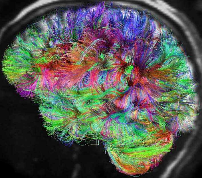Above image borrowed from Discover Magazine: http://discovermagazine.com/2013/jan-feb/36-new-project-maps-the-wiring-of-the-mind

On the cognative scale:

The brain is continually processing large amounts of information in parallel.
It is also continually collating information and learning about the past, present and future.

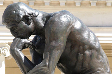Image borrowed from Wikimedia Commons: http://commons.wikimedia.org/wiki/File:Auguste_Rodin-The_Thinker-Legion_of_Honor-Lincoln_Park-San_Francisco.jpg

So what does this mean for us as data scientists and neural engineers?

Methods for modeling and classifying EEG signals should be

robust to noise
able to model spatial patterns (across electrode sites)
able to model temporal patterns (over the course of time)

I posit that Artificial Neural Networks (ANN) and, specifically, Recurrent Artificial Neural Networks (RNN), are well-suited for this role.

In this talk we will begin to explore methods for capturing spatiotemporal information using neural nets and give some examples of how this can be used to analize EEG signals.

Although we are focusing on EEG, these methods should be generally useful for analyzing other time-series and time-varying signals

Let's begin with some prerequisites.

# plotting
%matplotlib inline
import matplotlib.pyplot as plt
from mpl_toolkits.axes_grid1.inset_locator import zoomed_inset_axes
from mpl_toolkits.axes_grid1.inset_locator import mark_inset

# animation
from JSAnimation.IPython_display import display_animation
from matplotlib import animation

# matrices
import numpy as np
import scipy.sparse as sparsem
import scipy.sparse.linalg as sparsela

# JavaScript object notation
import json

# bandpass filtering, should be in tarball
import bandpass as bp

def addBias(m):
    """Add a column of ones for a bias term.
    """
    m1 = np.empty((m.shape[0], m.shape[1]+1))
    m1[:,:-1] = m
    m1[:,-1] = 1.0
    return m1

def loadData(fileName='s20-gammasys-gifford-unimpaired.json'):
    """Load some resting state EEG data.
    """
    dataHandle = open(fileName, 'r')
    data = json.load(dataHandle)
    dataHandle.close()

    data = data[0] # pull out resting state session
    sampRate = data['sample rate']
    chanNames = data['channels']
    nChan = len(chanNames)
    sig = np.array(data['eeg']['trial 1']).T
    sig = sig[:,:nChan] # omit trigger channel

    return sig, chanNames, sampRate

$\newcommand{\transpose}{\mathsf{T}}$ $\newcommand{\Mat}[1]{\mathbf{#1}}$

Next, let's generate some data to play with. Rows are observations and columns are channels.

sig is the signal we are interested in exploring. In this case, we examine 10 seconds of resting-state EEG. A bandpass filter is applied from 1-12Hz. This gives us a relatively smooth signal. In more realistic applications, we would want a wider passband.

time is simply a column vector $\left[ 1, \ldots, N \right]^\transpose$ denoting each timestep of our signal.

window gives the indices for the first 3 seconds of data. We will use this window to train our models and the remaining data to examine generalization.

if False:
    # sinusoid data for testing
    time = np.arange(0.0, 20.0*np.pi, 0.1)[:,None]
    sig = np.sin(time) #+ np.random.normal(scale=0.15, size=tFull.shape)
    window = np.arange(int((4.0*np.pi)/0.1))
else:
    # EEG data
    sig, chanNames, sampRate = loadData()
    filt = bp.IIRFilter(1.0, 12.0, sampRate=sampRate, order=3)
    sig = filt.filter(sig)
    sig = sig[:(10.0*sampRate),:]
    time = np.arange(0.0, 10.0, 1.0/sampRate)[:,None]
    winWidth = 2.0
    window = np.arange(int(winWidth*sampRate))

# for separating signal channels
scale = np.max(np.abs(sig))
sep = np.arange(sig.shape[1]) * 2.0 * scale

fig = plt.figure(figsize=(11,8))
ax = fig.add_subplot(1,1,1)
ax.plot(time, sig+sep[None,:])
ax.set_yticks(sep)
ax.set_yticklabels(chanNames)
ax.set_xlabel('Time (s)')
ax.autoscale(tight=True)

# zoomed inset plot
subx1,subx2 = (0.0,winWidth)
#suby1,suby2 = (-scale,sep[-1]+scale)
suby1,suby2 = (-scale,scale)
axins = zoomed_inset_axes(ax, zoom=4.0,
            bbox_to_anchor=(-1.0,sep[-1]),
            bbox_transform=ax.transData)
axins.plot(time[window], sig[window]+sep[None,:])

axins.set_xlim(subx1,subx2)
axins.set_ylim(suby1,suby2)
axins.get_xaxis().set_visible(False)
axins.get_yaxis().set_visible(False)
mark_inset(ax,axins, loc1=3, loc2=1, fc="none", ec="0.5");

# standardize using training data
time -= np.mean(time[window], axis=0)
time /= np.std(time[window], axis=0)
sig -= np.mean(sig[window], axis=0)
sig /= np.std(sig[window], axis=0)

First, let's look at the style of two-layer neural nets that we have already talked about. An example of such a network is depicted below.

Say that the network inputs are concatenated into a matrix $\Mat{X}$ with rows being observations and columns being dimensions. Also, let $\Mat{H}$ and $\Mat{V}$ be the weight matrices for the hidden and visible layers, respectively, and $\phi$ be our choice of sigmoid. The output of the network's hidden layer is

$\Mat{Z} = \phi(\Mat{\bar{X}}\Mat{H})$

and the final network output is

$\Mat{Y} = \Mat{\bar{Z}}\Mat{V}$

where a bar above a matrix denotes that a column of ones has been added for a constant bias term. These equations are also known as the forward pass.

Since these networks are directed and acyclic, they have a topological ordering. This means that they can be arranged so that all connections move in the forward direction from one layer to the next. For this reason, they are referred to as feedforward networks.

Below, we have a simple implementation of a two-layer feedforward network that is trained using stochastic gradient descent.

class FFNN(object):
    """Feed-Forward Neural Network
    """
    def __init__(self, x, g, nHidden=10, *args, **kwargs):
        self.nIn = x.shape[1]
        self.nOut = g.shape[1]
        self.nHidden = nHidden

        hwRange = np.sqrt(3.0 / (self.nIn+1))
        self.hw = np.random.uniform(-hwRange, hwRange,
            size=(self.nIn+1, self.nHidden))

        vwRange = np.sqrt(3.0 / (self.nHidden+1))
        self.vw = np.random.uniform(-vwRange, vwRange,
            size=(self.nHidden+1, self.nOut))

        self.train(x, g, *args, **kwargs)

    def eval(self, x):
        x1 = addBias(x)
        z = np.tanh(x1.dot(self.hw))
        z1 = addBias(z)
        return z1.dot(self.vw)

    def error(self, x, g):
        y = self.eval(x)
        return np.mean((g-y)**2)

    def grad(self, x, g):
        x1 = addBias(x)
        z  = np.tanh(x1.dot(self.hw))
        z1 = addBias(z)
        zPrime = 1.0-z**2
        y = z1.dot(self.vw)
        delta = 2.0 * (y - g) / g.size

        hg = x1.T.dot(delta.dot(self.vw[:-1,:].T) * zPrime)
        vg = z1.T.dot(delta)

        return hg, vg

    def train(self, x, g, hLearn=0.15, vLearn=0.1, learnDecay=0.0,
              batchSize=30, iterations=2000, verbose=False):
        for i in xrange(iterations):
            if verbose:
                print i, self.error(x, g), np.array((hLearn, vLearn)) * np.exp(-i*learnDecay)
            indices = np.random.permutation(np.arange(x.shape[0]))[:batchSize]
            hg, vg = self.grad(x[indices,:], g[indices,:])
            self.hw[...] -= hg * hLearn * np.exp(-i*learnDecay)
            self.vw[...] -= vg * vLearn * np.exp(-i*learnDecay)

Next, let's use our feedforward network to fit our EEG signal in the same fashion that we have fit curves before. So, the elements of the input matrix are time,

$\Mat{X}_{t,1} = t$

for $t = 1, \ldots, N$, where $N$ is the length of our training signal. The elements of the target matrix are then the signal values,

$\Mat{G}_{t,i} = \Mat{s}_i(t)$,

for each channel indexed by $i = 1, \ldots, 8$ and where $\Mat{s}(t)$ is the row vector of EEG signal voltages at time $t$.

xFull = time
gFull = sig

x = xFull[window]
g = gFull[window]
t = time[window]

net = FFNN(x, g, nHidden=30, hLearn=0.7, vLearn=0.6, learnDecay=3.0e-5,
           batchSize=50, iterations=40000, verbose=False)
print net.error(x, g)

yFull = net.eval(xFull)
y = yFull[window]

fig = plt.figure(figsize=(11,8))
ax = fig.add_subplot(111)

gline, = ax.plot(t, g[:,1], linewidth=3, color='blue')
yline, = ax.plot(t, y[:,1], linewidth=2, color='red')
ax.set_ylim(-2.5, 2.5)

def update(win):
    x = xFull[win]
    g = gFull[win]
    t = time[win]
    y = yFull[win]

    gline.set_ydata(g[:,1])
    gline.set_xdata(t)

    yline.set_ydata(y[:,1])
    yline.set_xdata(t)

    ax.set_xlim((t[0], t[-1]))
    return gline, yline, ax

def dataGen(win):
    win = np.array(win, copy=True)
    def dataGenWrapped(win=win):
        #while win[-1]+3 < len(x):
        while True:
            win += 20
            if win[-1] >= len(xFull):
                win -= win[0]
            yield win
    return dataGenWrapped

ani = animation.FuncAnimation(fig, update, dataGen(window), interval=80)
display_animation(ani, default_mode='once')

0.250105932159

With enough hidden units and training iterations, we are able to fit the major peaks of our signal (we could probably do better if we tweaked the parameters more). This model does not, however, generalize to the rest of our test signal. This is becuase our model only learned to map a short range of time values to signal outputs. Since our model begins to fall apart outside the training window, we say it is sensitive to shifts in time.

Note: the order in which the $x_i$'s are presented to the network doesn't matter. The network always gives the same static output.

So how can we model time-series and signals?

In order to model time-varying signals, a better approach is to look at the signal at each timestep and attempt to predict future signal values using information about the signal's past. This is called forecasting.

A common method for capturing temporal information in a signal is to incorporate a number of past signal values into the network's input at each timestep. This approach is known as time-delay embedding (TDE). The number of past values that are included in each network input is known as the embedding dimension. Consider the example below where $a$ is a simple linear signal and we embed 3 timesteps into each observation of our embedded signal.

def tde(m, embedDim=2):
    """Time-delay embedding.
    """
    s = []
    l = m.shape[0]
    for i in xrange(embedDim):
        s += [m[i:(l-embedDim+i),:]]
    return np.hstack(s)

a = np.arange(12).reshape((-1,1), order='F')
a

array([[ 0],
       [ 1],
       [ 2],
       [ 3],
       [ 4],
       [ 5],
       [ 6],
       [ 7],
       [ 8],
       [ 9],
       [10],
       [11]])

tde(a, 3)

array([[ 0,  1,  2],
       [ 1,  2,  3],
       [ 2,  3,  4],
       [ 3,  4,  5],
       [ 4,  5,  6],
       [ 5,  6,  7],
       [ 6,  7,  8],
       [ 7,  8,  9],
       [ 8,  9, 10]])

Since TDE simply embeds past values into each timestep, it can be combined with our feedforward networks (or other approaches) to create a model that is not sensitive to shifts in time. Let's give it a try! This time we try and predict the signal $\rho$ steps ahead using $d$ past values along with the same feedforward neural network architecture as before.

Let's denote our time-delay embedded signal by $\Mat{\hat{s}}^d(t)$. Then the elements of the input matrix are now

$\Mat{X}_{t,j} = \Mat{\hat{s}}^d_j(t)$

for $t = 1, \ldots, N-\rho-d$ and $j = 1, 2, \ldots, 8d$. The elements of the target matrix are now

$\Mat{G}_{t,i} = \Mat{s}_i(t+\rho+d)$.

embedDim = 10
shift = 3

xFull = tde(sig, embedDim)[:-(shift+embedDim)]
gFull = sig[(shift+embedDim):]

x = xFull[window]
g = gFull[window]
t = time[window]

net = FFNN(x, g, nHidden=10, hLearn=0.6, vLearn=0.4, learnDecay=2.0e-4,
           batchSize=50, iterations=4000)
print net.error(x, g)

yFull = net.eval(xFull)
y = yFull[window]

fig = plt.figure(figsize=(12,8))
ax = fig.add_subplot(111)

gline, = ax.plot(t, g[:,1], linewidth=3, color='blue')
yline, = ax.plot(t, y[:,1], linewidth=2, color='red')
ax.set_ylim(-2.5, 2.5)

def update(win):
    x = xFull[win]
    g = gFull[win]
    t = time[win]
    y = yFull[win]

    gline.set_ydata(g[:,1])
    gline.set_xdata(t)

    yline.set_ydata(y[:,1])
    yline.set_xdata(t)

    ax.set_xlim((t[0], t[-1]))
    return gline, yline, ax

ani = animation.FuncAnimation(fig, update, dataGen(window), interval=100)
display_animation(ani, default_mode='once')

0.0279851635833

Our model is now able to track the test signal with reasonable accuracy. Again, we could probably do better if we fine-tuned the hyper-parameters and used a validation set to regularize our model.

So why not call it a day?

There are several reasons why we might want to continue exploring other approaches:

Length of temporal patterns is limited by embedding dimension (Finite Impulse Response)
Potentially high dimensional input space for large embedding dimension
Does not appear to be how biological neural networks function

Another possibility is to incorporate feedback connections into our network, also known as recurrent connections. Recurrent networks have a cyclic architecture that gives them the ability to incorporate information from past inputs without using TDE. In other words, recurrent networks are capable of achieving memory.

In fact, while feedforward networks have been theoretically shown to be universal approximators of functions, recurrent networks have been theoretically shown to be universal approximators of finite state machines.

Elman Recurrent Neural Networks (ERNN) are a common type of recurrent network. ERNN have recurrent connections with a single timestep delay in the hidden layer only, as depected below. The forward pass for the hidden layer is

$\Mat{z}(t) = \phi(\Mat{\bar{x}}(t)\Mat{H} + \Mat{z}(t-1)\Mat{R})$

where $\Mat{R}$ is the adjacency matrix of recurrent weights. At any given time the state of an ERNN is defined by $\Mat{z}(t)$, which is referred to as the network context.

If we accumulate our $\Mat{z}(t)$ into a matrix $\Mat{Z}$, then the forward pass for our visible layer is the same as it was for our feedforward network,

$\Mat{Y} = \Mat{\bar{Z}}\Mat{V}$.

Note: the order in which the observations is presented matters!

Since ERNN have an intrinsic memory, TDE is not necessary. So, we can forecast a signal $\rho$ steps ahead in time by letting the input to the matrix at each timestep simply be the current signal value,

$\Mat{X}_{t,i} = \Mat{s}_i(t)$

and our target matrix be the signal value shifted $\rho$ steps ahead,

$\Mat{G}_{t,i} = \Mat{s}_i(t+\rho)$

for $t = 1, \ldots, N-\rho$.

Training ERNN can, however, be tricky. One approach is to unroll the network a number of steps through time so that it becomes a multi-layer network with inputs at each layer and with identical weights in each hidden layer, as illustrated below. The gradient can then be computed as it would with a feedforward network. The network can then be rolled back up by summing the contributions to the gradient from each layer. This process is known as backpropagation through time (BPTT).

Notice any similarities to the above diagram and some of the networks we have already looked at?

This is very similar to a deep network! This means that BPTT suffers from the same vanishing gradient problem. Unfortunately, the fact that all the layers must have the same weights prevents us from pre-training each layer incrementally. Also, since the order of the inputs matters, it is difficult to apply stochastic gradient descent.

I will leave it at this for now. The topic of my Master's thesis involved ERNN if anyone is interested. I think that there are many unanswered questions related to these networks... how can we apply the principals we have learned from deep feedforward networks?

Are there any alternatives?

A relatively new type of recurrent network, known as reservoir networks, were proposed independently by Herbert Jaeger and Wolfgang Mass circa 2000. These networks can be trained quickly using a relatively simple scheme. In particular, we will look at a type of recurrent network known as Echo State Networks (ESN).

ESN have an architecture that is similar to ERNN, depicted below, but with a relatively large and sparsely connected hidden layer, called a reservoir. Sparsity encourages the reservoir to produce a large variety of loosely related outputs, called the reservoir activations.

The equations for the forward pass of an ESN are the same as for ERNN, as are our input and target matrices.

The training procedure for ESN is remarkably simple. The reservoir weights are first initialized to random values from the uniform distribution and then scaled in a way that achieves the Echo State Property (ESP). Briefly stated, a reservoir is said to possess the ESP if the effect on the reservoir activations caused by a given input fades as time passes. The ESP also implies that the outputs produced by two identical ESN will converge toward the same sequence when given the same input sequence, regardless of the starting network context.

A rule of thumb for attaining the ESP (although not a sufficient condition) is to scale the reservoir so that the magnitude of its largest eigenvalue, also as the spectral radius, is less than one. Let us denote our initial reservoir weight matrix by $\Mat{R}_0$ and say that the spectral radius of $\Mat{R}_0$ is $\lambda_0$. Then our final reservoir weight matrix is

$\Mat{R} = \frac{\lambda_\phantom{0}}{\lambda_0} \Mat{R_0}$

where $\lambda$ is the desired spectral radius of the reservoir.

Since the weights of our reservoir are fixed and the visible layer is linear, the our visible weights can be found using linear regression. We use ridge regression to allow regularization. First, we accumulate all of our reservoir activations for the training signal into the rows of a matrix $\Mat{A}$. We then solve for our visible weights using the standard equation for ridge regression,

$\Mat{V} = ( \bar{\Mat{A}}^\transpose \bar{\Mat{A}} + \Mat{\Gamma} )^{\ast} \bar{\Mat{A}}^\transpose\Mat{G}$

where $^\ast$ denotes the Moore-Penrose pseudoinverse and $\Mat{\Gamma}$ is a square matrix with the ridge regression penalty, $\gamma$, along the diagonal except with a zero in the last entry to avoid penalizing the bias term.

Below, we see an implementation of a simple ESN. Note that it uses the scipy.sparse package to improve performance through a sparse matrix representation for the reservoir and computing eigenvalues.

class ESN(object):
    """Echo State Network
    """
    def __init__(self, x, g, inRange=0.3, inConn=0.2,
                 nRes=1000, spectralRadius=0.9, resConn=0.01,
                 *args, **kwargs):
        self.nIn = x.shape[1]
        self.nOut = g.shape[1]
        self.nRes = nRes

        inWeights = np.random.uniform(-inRange, inRange, size=(self.nIn+1, self.nRes))
        connMask = np.random.random(inWeights.shape) > inConn
        inWeights[connMask] = 0.0

        resWeights = np.random.uniform(-1.0, 1.0, size=(self.nRes, self.nRes))
        connMask = np.random.random(resWeights.shape) > resConn
        resWeights[connMask] = 0.0

        l = np.abs(sparsela.eigs(sparsem.csc_matrix(resWeights), k=1,
                   which='LM', tol=0.0001, return_eigenvectors=False))[0]
        resWeights[:,:] *= spectralRadius / l

        self.hw = np.vstack((inWeights, resWeights))
        self.hw = sparsem.csc_matrix(self.hw)

        self.train(x, g, *args, **kwargs)

    def evalRes(self, x, nIterate=0, iterateShift=1):
        nObs = x.shape[0]
        x1 = addBias(x)

        act = np.empty((nObs+nIterate, self.nRes))
        context = np.zeros(self.nRes)
        xs = np.empty((1,x1.shape[1]+context.shape[0]))

        hwt = self.hw.T
        for s in xrange(nObs+nIterate):
            if s < nObs:
                xs[:,:x1.shape[1]] = x1[s,:]
            else:
                feedback = np.append(act[s-iterateShift,:],1.0).dot(self.vw)
                feedback1 = np.append(feedback, 1.0)
                xs[:,:x1.shape[1]] = feedback1
            xs[:,x1.shape[1]:] = context

            context[:] = np.tanh(hwt.dot(xs.T).T)
            act[s,:] = context

        return act

    def eval(self, x, nIterate=0, iterateShift=1):
        act = self.evalRes(x, nIterate=nIterate, iterateShift=iterateShift)
        act1 = addBias(act)
        return act1.dot(self.vw)
    
    def error(self, x, g):
        y = self.eval(x)
        return np.mean((g-y)**2)

    def train(self, x, g, penalty=0.0):
        act = self.evalRes(x)
        act1 = addBias(act)
        
        penaltyMat = penalty * np.eye(act1.shape[1])
        penaltyMat[-1,-1] = 0.0
        
        self.vw, resid, rank, s = \
            np.linalg.lstsq(act1.T.dot(act1) + penaltyMat, act1.T.dot(g))

Applying our ESN to our example, we see that they are very fast to train and appear to perform comparably to feedforward nets with TDE, if not better.

nRes = 1000
spectralRadius = 0.9
penalty = 5.0
shift = 3

xFull = sig[:-shift]
gFull = sig[shift:]

x = xFull[window]
g = gFull[window]
t = time[window]

net = ESN(x, g, nRes=nRes, spectralRadius=spectralRadius, penalty=penalty)
print net.error(x, g)

yFull = net.eval(xFull)
y = yFull[window]

fig = plt.figure(figsize=(12,8))
ax = fig.add_subplot(111)

gline, = ax.plot(t, g[:,1], linewidth=3, color='blue')
yline, = ax.plot(t, y[:,1], linewidth=2, color='red')
ax.set_ylim(-2.5, 2.5)

def update(win):
    x = xFull[win]
    g = gFull[win]
    t = time[win]
    y = yFull[win]

    gline.set_ydata(g[:,1])
    gline.set_xdata(t)

    yline.set_ydata(y[:,1])
    yline.set_xdata(t)

    ax.set_xlim((t[0], t[-1]))
    return gline, yline, ax

ani = animation.FuncAnimation(fig, update, dataGen(window), interval=100)
display_animation(ani, default_mode='once')

0.00995120105488

These networks are great for forecasting, but can we do longer-term predictions?

Long-term prediction is the holy-grail of time-series analysis and it is typically very challenging. In some of our recent work, we have explored the ability of ELRNN and ESN to perform long-term prediction of EEG signals and have found some interesting results.

This is achieved using what is known as an iterated model. An iterated model is formed placing a feedback loop from the network outputs back into the network inputs so that the network takes its previous predictions as input instead of the true signal values. Typically, the network begins by using the true signal and then transitions to an iterated model at some point in time so that

$\Mat{y}(t) = \left\{ \begin{array}{ll} \textit{net}(\Mat{s}(t-1)), & \textrm{if } \; t < M \\ \textit{net}(\Mat{y}(t-1)), & \textrm{otherwise,} \end{array} \right.$

where $\textit{net}$ denotes the forward pass of our network and $M$ is the time at which we transition to an iterated model.

Below, see see a quick example of the signal generated using an iterated ESN. The signal begins by running over the training signal and transitions to an iterated model once it reaches the test signal.

nRes = 1000
spectralRadius = 0.99
penalty = 1.0
shift = 1

xFull = sig[:-shift]
gFull = sig[shift:]

x = xFull[window]
g = gFull[window]
t = time[window]

net = ESN(x, g, nRes=nRes, spectralRadius=spectralRadius, penalty=penalty)
print net.error(x, g)

yFull = net.eval(x, nIterate=len(xFull)-len(x), iterateShift=shift)
y = yFull[window]

fig = plt.figure(figsize=(12,8))
ax = fig.add_subplot(111)

gline, = ax.plot(t, g[:,1], linewidth=3, color='blue')
yline, = ax.plot(t, y[:,1], linewidth=2, color='red')
ax.set_ylim(-3, 3)

def update(win):
    x = xFull[win]
    g = gFull[win]
    t = time[win]
    y = yFull[win]

    gline.set_ydata(g[:,1])
    gline.set_xdata(t)

    yline.set_ydata(y[:,1])
    yline.set_xdata(t)

    ax.set_xlim((t[0], t[-1]))
    return gline, yline, ax

ani = animation.FuncAnimation(fig, update, dataGen(window), interval=100)
display_animation(ani, default_mode='once')

0.000233693669271

How can we use these models to analyze EEG?

There are lots of possibilities, but I have been considering two applications.

generative classifiers
causality and functional connectivity (kaggle competition)